Lagrange Interpolation Polynomials

If we wish to describe all of the ups and downs in a data set, and hit every point, we use what is called an interpolation polynomial. This method is due to Lagrange.

Suppose the data set consists of  N  data points:

(x₁, y₁), (x₂, y₂), (x₃, y₃), ..., (x_N, y_N)

The interpolation polynomial will have degree  N – 1 . It is given by:

P(x) = j₁(x) y₁ + j₂(x) y₂ + j₃(x) y₃ + ... + j_N(x) y_N

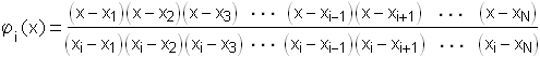
where the functions  j_i(x)  (i = 1, 2, 3, ..., n)  are given by:

Don't fret! This is easier than it looks. The key thing to notice is that the numerator of  j_i(x)  contains the entire sequence of factors  (x – x₁), (x – x₂), (x – x₃), ... (x – x_N), with the exception of the single factor  (x – x_i). Likewise, the denominator contains the entire sequence of factors  (x_i – x₁), (x_i – x₂), (x_i – x₃), ... (x_i – x_N), with the exception of the single factor  (x_i – x_i).

Now notice:  j_i(x_i) = 1  (numerator = denominator), but  j_i(x_j) = 0  (numerator = 0, since it contains the factor  (x_j – x_j) ) for any  j  not equal to  i . This means that  P(x_i) = y_i , which is exactly what we want!

If this seems like smoke and mirrors, consider a simple example. Here's the data for  g  again:

x	g(x)
0	–250
10	0
20	50
30	–100

In this case there are  N = 4  data points, so we will create a polynomial of degree  N – 1 = 3 . We have  x₁ = 0 ,  x₂ = 10 ,  x₃ = 20 ,  x₄ = 30 , and  y₁ = –250 ,  y₂ = 0 ,  y₃ = 50 ,  y₄ = 100 . So:

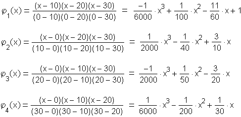
Multiplying each of these by the appropriate  y_i   (i = 1, 2, 3, 4)  and adding together the terms of like power then gives:

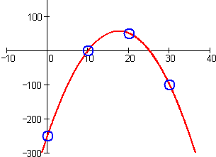
The cubic terms cancel, and we arrive at a simple quadratic description of the data.

A quick plot of the data together with the polynomial shows that it indeed passes through each of the data points:

For an interactive demonstration of Lagrange interpolation polynomials, showing how variations in the data points affect the resulting curve, go here.