Linear Functions

Numeric Representation

x g(x) 0 0.27 10 0.55 20 0.83 30 1.11

x h(x) 0 1.44 2 3.34 7 8.09 10 10.94

To recognize a linear trend in a data set, we make use of the key algebraic property of linear functions  f(x) = a + bx . Namely:

We can read this equation this way: If the input  x  is increased by a constant interval (Dx), then the output  f(x)  will also increase by a constant interval (bDx).

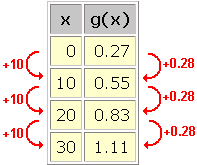
For data sets with constant intervals between inputs, this is an easy pattern to recognize:

In this data set, we see a linear trend with  Dx = 10  and  bDx = 0.28 . Thus, the data may be represented by a linear function with slope  b = 0.28/10 = 0.028 . The y-intercept  a  appears explicitly in the data set: 0.27 . If the y-intercept had not appeared explicitly – say the data began at  x = 10  – then we could have pluggged in any data point and solved for  a . For example,

f(10) = a + (0.028)(10) = 0.55

a = 0.55 – (0.028)(10) = 0.27

We arrive at the following model for this data set:

g(x) = 0.27 + (0.028)x

This equation can be used to interpolate or extrapolate further data values.

What if a data set has not been recorded at equal intervals of the input? We can rewrite the key algebraic property this way:

This form of the equation can be read: Whatever the increase in input (Dx) between two data points, the slope remains constant (b).

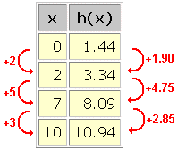
We can recognize this pattern even in data sets without constant intervals between the inputs:

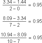
Nothing looks constant at first, but when we calculate the slopes we find:

The constant slope  b = 0.95  is hiding in the data. We find the y-intercept  a = 1.44  as above, and model this data with the linear equation:

h(x) = 1.44 + (0.95)x