Rational Functions

Numeric Representation

x g(x)
0 31
10 32
20 33
30 35
40 40
50 55
60 456
70 153
80 49
90 35
100 33
 

Certain algebraic properties distinguish rational functions from polynomials, and we can look for these in data sets to see if we should consider a rational model.

One property of rational functions is the presence of singularities. In data, we can recognize a singularity by the very large output values, either positive or negative, in their immediate vicinity. Large values of opposite sign near the input  x = a  might lead us to a rational model with a factor of  (x – a)  in the denominator. Large values of the same sign in the vicinity of the input  x = a  might lead us to a rational model with a factor of  (x – a) 2  in the denominator.

Not all rational functions have singularities, however. For example, a data set modeled by the following function would not display any large output values:

Another property of rational functions is the presence of asymptotes. When a data set displays a recognizable horizontal asymptote, with outputs that "level off" at some fixed value, the behavior can not be described by a polynomial. Output values that level off at  y = 0  might lead us to a rational model with a denominator of higher degree than the numerator. Output values that level off at  y = A  might lead us to a rational model with a numerator and denominator of the same degree, and coefficients in a ratio of  A  for the highest powers.

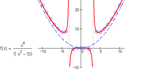
Not all rational functions have horizontal asymptotes, however. If a data set has an underlying trend that is modeled by a rational function with a numerator of higher degree than the denominator, then the long term behavior will resemble a power function – just like a polynomial. For example, the function below becomes indistinguishable from the quadratic power  x2/5  in the long term:
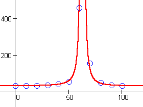
In the data for  g  above, something singular seems to occur between  x = 60  and  x = 70 . The output values climb to uncharacteristic highs, relative to the rest of the data. Since the values are higher at  x = 60  than they are at  x = 70 , we would expect that any singularity lies closer to  x = 60 . We might put a factor of, say,  (x – 63)  in the denomitator of our rational model. Since the outputs are of the same sign on either side of the singularity, we would want to square this factor.

We also notice that the data seems to level off around  y = 30  as we move away from the singularity in either direction. To model this, we might include a highest power of  30 x 2  in the numerator to balance the  (x – 63) 2  in the denominator.

If we graph  g(x) = (30 x 2 + a x + b) / (x – 63) 2  together with the data, and adjust  a  and  b , we find that values of  a = –3800  and  b = 125000  give a reasonable model of the data's overall behavior:

 
Back to Contents