Trigonometric Functions

Numeric Representation

x g(x) 0 2.02 2 5.38 7 3.14 10 4.52 13 2.63 18 1.78 20 4.00 24 2.01 27 5.23 29 4.24 33 4.80

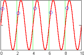
Trigonometric functions model data with periodic trends. Even if a data set can be accurately represented by a periodic function, however, we may not be able to recognize this by looking for repetitions in the output values. This is because our data collection may be sampling the underlying periodic function at intervals which are not representative of the actual period. For example, the following data points are obtained by sampling a function with a period of  2 . Because our sampling comes at irregular intervals, the output values seem to jump up and down with no discernable repetitions:

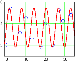
Likewise, although the following data points are collected at regular intervals, sampling the same function as above, the outputs indicate a period of  4 , not  2 . Moreover, they completely misrepresent the size of the underlying fluctuations:

The difficulties involved in obtaining representative samples of periodic phenomena are really problems of science, not mathematics. If we are presented with a data set that varies up and down within some fixed range of outputs, then there is a good chance that we will be able to find a periodic model of it. The model may give an accurate description of the data without necessarily giving an accurate description of the underlying pattern in nature that produced it.

Consider the data for  g , above. The output values vary between a low of  1.78  and a high of  5.38 . They go up and down without a discernable pattern, but there is no tendency, at least in the interval sampled, for the data to grow large, grow small, or approach an asymptote. We might try a trigonometric model.

The sine function  y = sin(x)  varies up and down around a midline at  y = 0  with an amplitude of  1 . The data has a larger amplitude, and it varies around a midline above  y = 0  (the outputs are never negative).

We can approximate the data's midline by taking an average value of the outputs. The result is  3.61 . A vertical translation of the sine function to  y = sin(x) + 3.61  gives us a model with a more appropriate midline.

The data values vary up to  5.38 – 3.61 = 1.77  above the midline, and up to  3.61 – 1.78 = 1.83  below the midline. We can approximate the amplitude by  1.8  and adjust our model using a vertical dilation to read  y = (1.8) sin(x) + 3.61 .

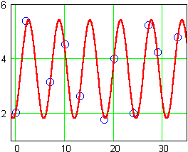
At this point, a plot of the data together with the model might be wise. It will tell us if we need to make further adjustments to the model using phase shifts or horizontal dilations:

The period looks approximately correct, so we will not need to alter it with any horizontal dilations. All of the data, however, seems to fall just a bit to the right of the model curve. If we incorporate a phase shift of  1  to the right, for a model function of  y = (1.8) sin(x – 1) + 3.61 , we arrive at a reasonable, rough-and-ready fit: