When answering the question How good is the fit?, we often start with a plot of the fitted curve through the data points. We can then tell "by eye" if the fit is at all close, or if it's out in left field.

Working "by eye," however, isn't very precise. You may fit a different curve than someone else – through the very same set of data points. And if you want to show that your fit is absolutely the "best" fit possible, "by eye" doesn't provide you with any quantitive measures for comparison.

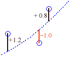
To measure precisely how good a particular fit is, we typically look at the residuals:

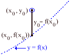
The residual for each data point measures how far it is (vertically) from the fitted curve. A positive residual means that the data point is above the fitted curve; a negative residual means that it is below. If a data point has coordinates  (x₀, y₀), and the corresponding point on the fitted curve  y = f(x)  has coordinates  (x₀, f(x₀)), then the residual is just the difference  y₀ – f(x₀) :

To measure how far off an entire data set is from a fitted curve, we might just add up all of the individual residuals. We'd think that a small sum of residuals would indicate a good fit.

Unfortunately, since some of the residuals may be positive and some of them may be negative, it is possible to get a small sum even when we don't have a good fit. This can happen if large positive residuals cancel out large negative residuals. E.g.:

1.2 + (-3.7) + 0.1 + 2.3 + (-0.8) + 0.9 = 0.

What we need to do is add up not the residuals, but something like the absolute value of the residuals, | y₀ – f(x₀) | . These numbers will always be positive, and they will not add up to something small unless each of them is small individually. We could add up the squares of the residuals, ( y₀ – f(x₀) ) ², to achieve the same effect.

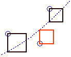
The latter approach is the traditional one. We measure the fit of a particular curve by adding up the squares of all of the residuals. If the sum is small, the fit is good. The method of picking the "best" fitting curve for a set of data by making this sum as small as possible is called the method of least squares.

The method of least squares picks the curve that makes the areas of the squares, shown below, as small as possible: