Logarithmic Functions
Numeric Representation
|
x
|
g(x)
|
|
0
|
–––
|
|
10
|
3.32
|
|
100
|
6.64
|
|
1000
|
9.97
|
|
|
|
x
|
h(x)
|
|
0
|
–––
|
|
2
|
–0.28
|
|
7
|
–0.78
|
|
10
|
–0.92
|
|
To recognize a logarithmic trend in a data set, we make use of the key algebraic property of logarithmic functions f(x) = a log b(x) . Namely:

We can read this equation this way: If the input x is increased by a constant multiple (k), then the output f(x) will increase by a constant interval (a log b(k)).
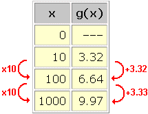
For data sets with constant multiples between inputs, this is an easy pattern to recognize:

In this data set, we see an approximately logarithmic trend with k = 10 and a log b(k) = 3.32 . Combining these two equations gives a log b(10) = 3.32 .
To find a and b , we need a second equation relating these variables. Plugging in any other data point, such as (100, 6.64) , seems like a good idea. We get a log b(100) = 6.64 . Unfortunately, this does not give us any additional information about a and b . If we use the laws of logarithms (see section on the algebraic representation of logarithmic functions), we see that:
a log b(100) = a log b(10 2) = 2 a log b(10) .
So saying that a log b(100) = 6.64 is the same as saying 2 a log b(10) = 6.64 , which is the same as saying a log b(k) = 3.32 ...which is the same as the previous data point!
The data point (1000, 9.97) likewise gives no new information (if we ignore the small difference in the last decimal place). In fact, no data point of the form (10 n, n(3.32)) will tell us anything that the first data point (n = 1) and the laws of logarithms couldn't have told us on their own.
This is an odd situation: The data tells us that the trend is logarithmic, but it does not give us enough information to determine a and b . The reason is that many different combinations of a and b will make f(x) = a log b(x) fit this data set.
For example, if we arbitrarily pick a = 1 (because it's simple), we get an equation involving b alone: log b(10) = 3.32 . In exponential form, this is b 3.32 = 10 . Thus b = (10) 1/(3.32) , which comes out to be just about 2 .
We have arrived at the following simple model for this data set:
g(x) = log 2(x)
Other models are g(x) = 2 log 4(x) and g(x) = 3 log 8(x) . Do you see why?
Working with inputs which are not constant multiples avoids the issue of redundant information in the data set. Recognizing a logarithmic trend isn't much more difficult in this case.
We saw above that an arbitrary choice of a = 1 will not affect our ability to find a model for the data. With this choice, we can rewrite the key property of logarithms as follows:
f(kx) – f(x) = log b(k)
In exponential form, this is:
b [f(kx) – f(x)] = k
Solving for b gives:
b = k 1/[f(kx) – f(x)]
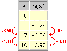
To recognize a logarithmic trend in an arbitrary data set, we look for the term on the right of this equation to remain constant for each pair of data points. That constant is b . Consider:

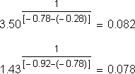
Calculating k 1/[f(kx) – f(x)] for consecutive pairs of ponts in this data set gives:

A constant base of b = 0.08 seems to be hiding in the data. We could approximately model this data set with the equation:
h(x) = log 0.08(x)
![]()

